Example
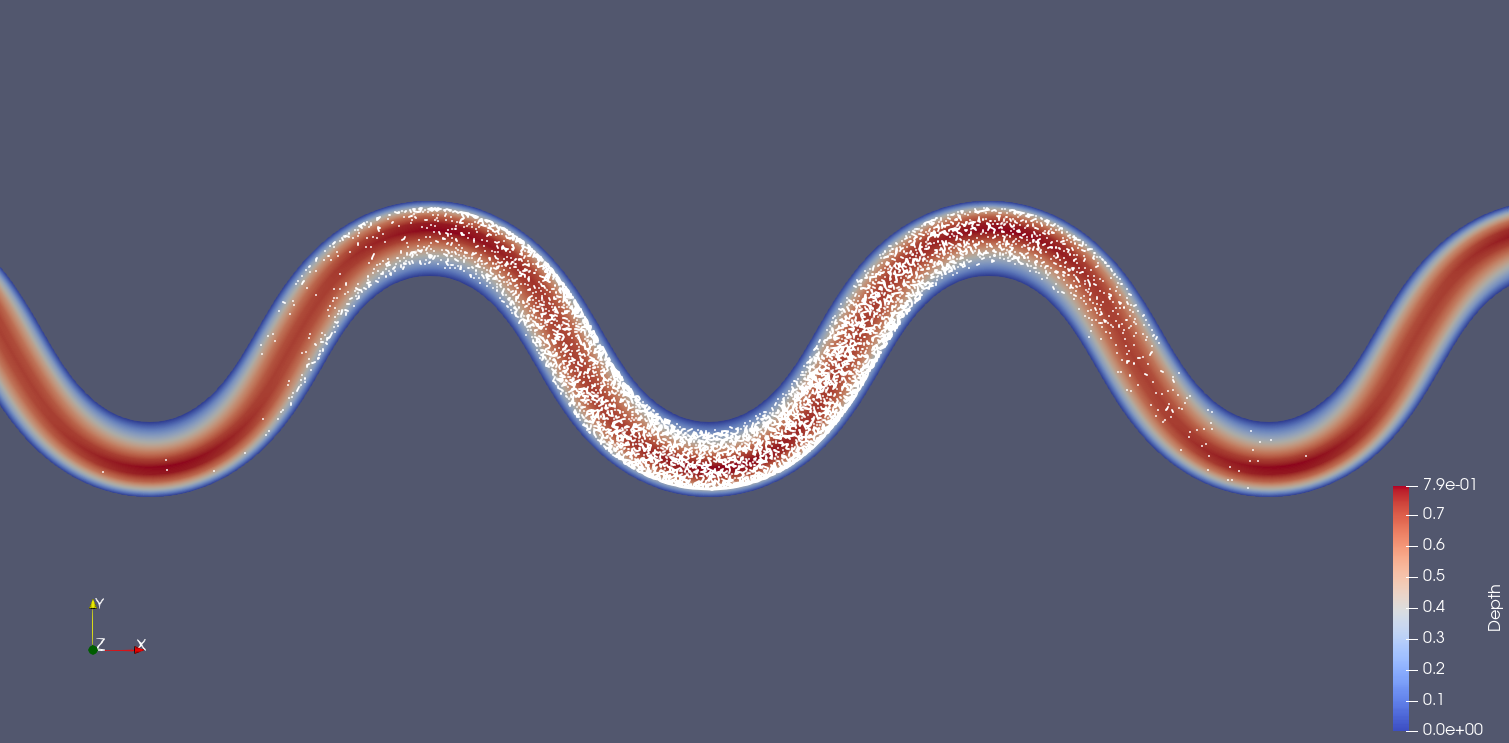
This simulation example releases 1000 particles from a point-source in an idealized meandering river.
Running from Command Line
First, create a configuration file. You can generate a template with:
fluvial_particle --init
Then edit the generated settings.toml file to match your simulation needs.
To run the simulation:
fluvial_particle settings.toml ./output
Which prints to stdout:
Beginning simulation
Using seed 54059
Simulating 1000 particles
Particle class: Particles
Velocity field will be interpolated from 3D grid
Simulation start time is 0.0, maximum end time is 1000.0, using timesteps of 0.25 (all in seconds).
Remaining time steps 3600/4000 || Elapsed Time: 0:00:02.532642 h:m:s || ETA 0:00:22.857252 h:m:s
Remaining time steps 3200/4000 || Elapsed Time: 0:00:05.175054 h:m:s || ETA 0:00:20.732601 h:m:s
Remaining time steps 2800/4000 || Elapsed Time: 0:00:07.856087 h:m:s || ETA 0:00:18.352711 h:m:s
Remaining time steps 2400/4000 || Elapsed Time: 0:00:12.652966 h:m:s || ETA 0:00:18.999232 h:m:s
Remaining time steps 2000/4000 || Elapsed Time: 0:00:16.042314 h:m:s || ETA 0:00:16.058364 h:m:s
Remaining time steps 1600/4000 || Elapsed Time: 0:00:19.357288 h:m:s || ETA 0:00:12.918307 h:m:s
Remaining time steps 1200/4000 || Elapsed Time: 0:00:22.243454 h:m:s || ETA 0:00:09.544262 h:m:s
Remaining time steps 800/4000 || Elapsed Time: 0:00:25.076732 h:m:s || ETA 0:00:06.278982 h:m:s
Remaining time steps 400/4000 || Elapsed Time: 0:00:27.967835 h:m:s || ETA 0:00:03.116172 h:m:s
Remaining time steps 0/4000 || Elapsed Time: 0:00:30.928731 h:m:s || ETA 0:00:00.007734 h:m:s
Finished simulation in 0:00:30.931503 h:m:s
Post-processing...
Finished in 0:00:30.968555 h:m:s
The output from the run can be visualized in Paraview by opening an XDMF file and reading it with the XDMF Reader. Here are the example outputs at t=500 seconds from the particles.xmf and cells2d.xmf files – in the first image, the mesh is colored by flow depth:
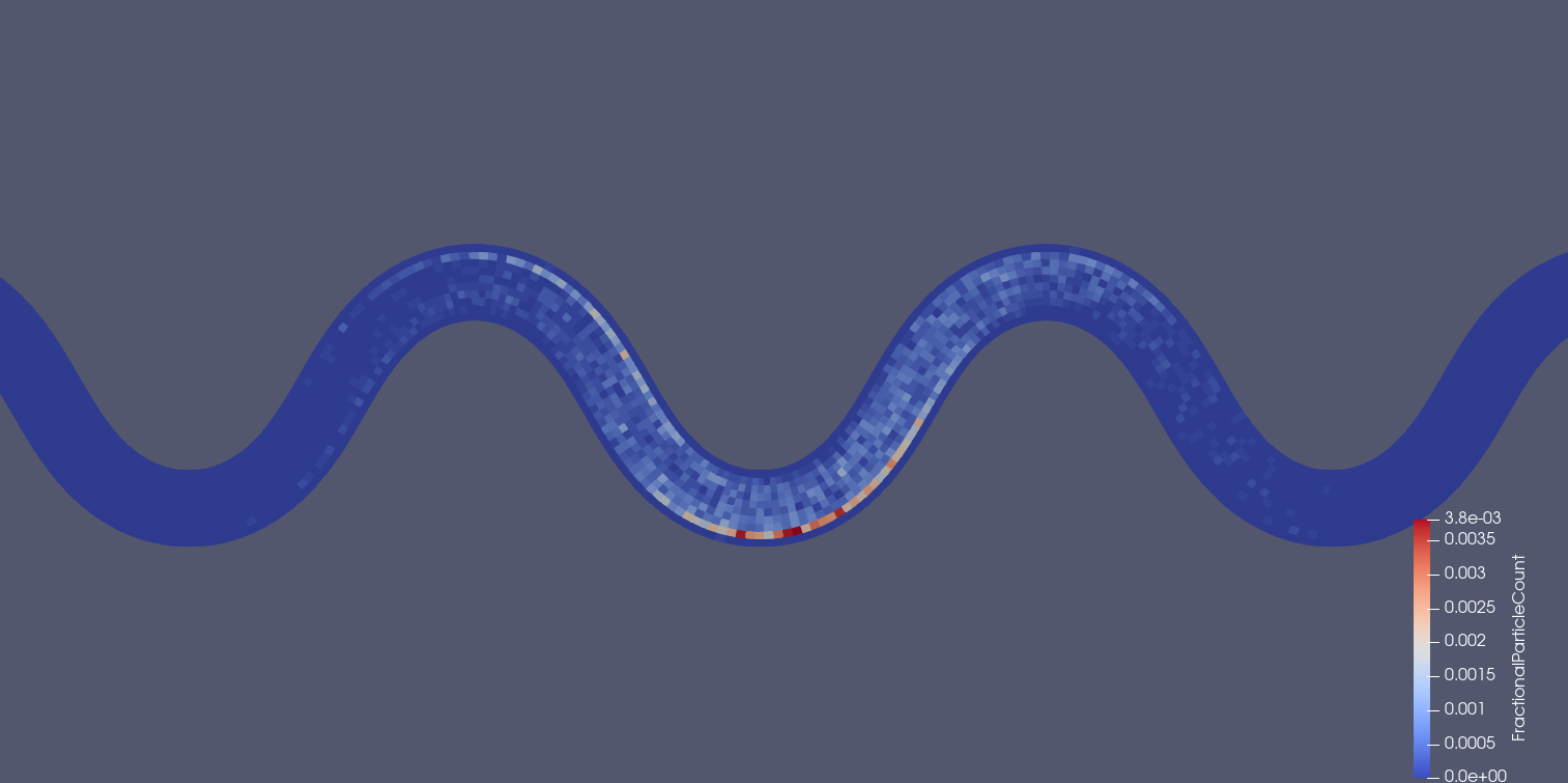
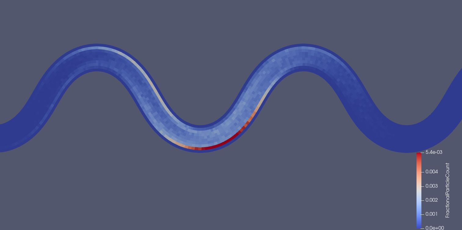
Notice the discontinuous concentrations in the cells2d.xmf plot. Additional simulated particles will tend to generate smoother concentration distributions. For instance, here are the 2D concentrations using 100,000 particles instead of 1,000 (which takes ~100x as long to simulate):
Running from Python/Notebooks
For Jupyter notebooks or Python scripts, use the programmatic API:
from fluvial_particle import get_default_config, run_simulation

# Get default configuration as a dictionary
config = get_default_config()

# Customize the configuration
config["simulation"]["time"] = 1000.0
config["simulation"]["dt"] = 0.25
config["simulation"]["print_interval"] = 10.0

config["particles"]["count"] = 1000
config["particles"]["start_location"] = [6.14, 9.09, 10.3]

config["grid"]["track_3d"] = True
config["grid"]["file_2d"] = "./tests/data/Result_FM_MEander_1_long_2D1.vtk"
config["grid"]["file_3d"] = "./tests/data/Result_FM_MEander_1_long_3D1_new.vtk"

# Run simulation directly with dict (no file needed)
results = run_simulation(config, output_dir="./output", seed=42)

# Access results
print(f"Simulated {results.num_particles} particles")
print(f"Over {results.num_timesteps} timesteps")
print(f"Times: {results.times[:5]}...")

# Get particle positions at final timestep
positions = results.get_positions(timestep=-1)
print(f"Final positions shape: {positions.shape}")

# Convert to DataFrame for analysis
df = results.to_dataframe(timestep=-1)
print(df.head())
Example TOML Configuration
This is the recommended configuration format for new projects:
# Fluvial-particle simulation configuration
# Meandering river example

[simulation]
time = 1000.0            # Maximum simulation time [seconds]
dt = 0.25                # Time step [seconds]
print_interval = 10.0    # Output interval [seconds]

[particles]
type = "Particles"
count = 1000             # Particles per processor
start_location = [6.14, 9.09, 10.3]

[particles.physics]
lev = 0.00025            # Reach-averaged lateral eddy viscosity

[grid]
track_3d = true
file_2d = "./tests/data/Result_FM_MEander_1_long_2D1.vtk"
file_3d = "./tests/data/Result_FM_MEander_1_long_3D1_new.vtk"

[grid.field_map_2d]
bed_elevation = "Elevation"
wet_dry = "IBC"
shear_stress = "ShearStress (magnitude)"
velocity = "Velocity"
water_surface_elevation = "WaterSurfaceElevation"

[grid.field_map_3d]
velocity = "Velocity"
Example Python Configuration (Legacy)
Python configuration files are still supported. Update "path/to/repo" with the correct path on your machine:
Note
This example uses legacy VTK (.vtk) files. For large meshes, consider using VTK XML (.vts) format which offers better compression and faster I/O. See the configuration file documentation for supported formats.
"""Options file for fluvial particle model."""
from fluvial_particle.Particles import Particles

# Required keyword arguments
file_name_2d = "path/to/repo" + "//tests/data/Result_FM_MEander_1_long_2D1.vtk"
file_name_3d = "path/to/repo" + "//tests/data/Result_FM_MEander_1_long_3D1_new.vtk"
SimTime = 1000.0
dt = 0.25
PrintAtTick = 10.0
Track3D = 1
NumPart = 1000
StartLoc = (6.14, 9.09, 10.3)
ParticleType = Particles

# Field name mappings (Delft-FM example)
field_map_2d = {
    "bed_elevation": "Elevation",
    "wet_dry": "IBC",
    "shear_stress": "ShearStress (magnitude)",
    "velocity": "Velocity",
    "water_surface_elevation": "WaterSurfaceElevation",
}
field_map_3d = {
    "velocity": "Velocity",
}

# Optional keyword arguments
lev = 0.00025  # reach-averaged lateral eddy viscosity